Probability Functions & Moments

Once you’ve constructed a model of \(p(t, v, \textbf{x}, z)\), popkinmocks provides tools to calculate its marginal and conditional probability functions, moments and covariances. These can be either light weighted or mass weighted.

Let’s take a look, using the mixture model saved in the Constructing Models page:

import numpy as np
import matplotlib.pyplot as plt
import dill
import popkinmocks as pkm
with open('data/my_mixture_component.dill', 'rb') as file:
    galaxy = dill.load(file)
cube = galaxy.cube

Probability Functions

All probability functions can be evaluated using a component’s get_p method. For example, to evaluate the marginal distribution

\[ p(z) = \int\int\int p(t, v, \textbf{x}, z) \;\mathrm{d}t \;\mathrm{d}v \;\mathrm{d}\textbf{x}. \]

do this,

p_z = galaxy.get_p('z')

while to evaluate the conditional distribution

\[ p(v|t) = \frac{p(v,t)}{p(t)} \]

do this

p_v_t = galaxy.get_p('v_t')
p_v_t.shape

(25, 9)

The shape of the returned array corresponds to the order of the variables in the input string. Rules for constructing valid strings accepted by get_p are below.

get_p accepts two optional keyword arguments:

• density determines whether a probability density is returned (True, by default) or an integrated probability (False)

• light_weighted (default False), see below for details.

So to evaluate light-weighted LOSVDs conditional on position, do this

p_v_x = galaxy.get_p('v_x', light_weighted=True, density=False)
p_v_x.shape

(25, 21, 21)

Since density=False, these should be close to one when summed over the velocity dimension,

np.allclose(np.sum(p_v_x, 0), 1.)

True

Mixture components can additionally take a third argument collapse_cmps (default True). If collapse_cmps=False, then the returned distribution is split by mixture components, e.g.

p_x = galaxy.get_p('x', light_weighted=True, density=False, collapse_cmps=False)
p_x.shape

(2, 21, 21)

The first dimension has size two corresponding to the two components in this mixture model. They are weighted by the mixture weights, so the total probability still sums to one,

np.sum(p_x)

np.float64(0.9999999999999996)

Lastly note there is an equivalent (and more numerically accurate) version get_log_p for evaluating log probabilities.

Distribution Strings & Shapes

Distributions are specified by a string. The rules for constructing these strings are:

• marginal distributions have no underscore

• conditional distributions have an underscore dividing dependent variables on the left and conditioners on the right

• variables must be in alphabetical order (on either side of the underscore, if present)

Some examples:

• tz \(\rightarrow p(t, z)\)

• vt invalid since not in alphabetical order

• xz_v \(\rightarrow (\textbf{x}, z | v)\)

• zx_v invalid since zx is not in alphabetical order

The order of dimensions in the arrays returned by get_p correspond to the order of the variables provided in the input string.

Moments

To evaluate moments e.g.

\[ \mathbb{E}(z) = \int z p(z) \;\mathrm{d}z, \]

do this

mean_z = galaxy.get_mean('z')
print(mean_z)

-0.10606818696102341

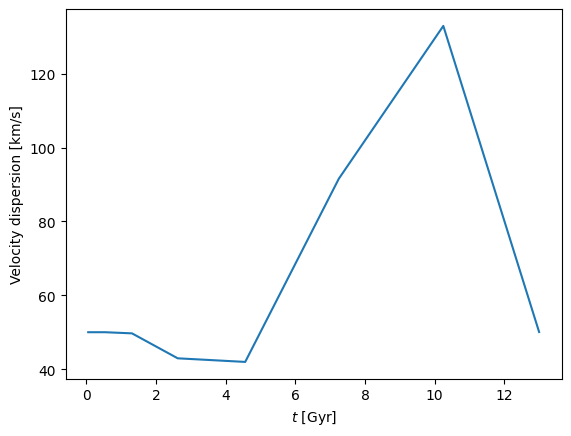
To calculate conditional moments e.g.

\[ \mathbb{Var}(v|t) = \int (v - \mathbb{E}(v|t))^2 p(v|t) \;\mathrm{d}v, \]

do this

var_v_t = galaxy.get_variance('v_t')
cube.plot('t', var_v_t**0.5)
_ = plt.gca().set_ylabel('Velocity dispersion [km/s]')

There are four main methods for evaluating moments:

• get_mean,

• get_variance,

• get_skewness,

• get_kurtosis, or get_excess_kurtosis,

while the method get_excess_central_moment can be used for arbitrary higher order.

Rules for constructing valid input strings are similar to those given above. One difference is that moments are only defined for distributions over one variable i.e. it makes sense to talk about the variance of \(p(z)\) but not of \(p(t,z)\) since we don’t know whether the variance is with respect to \(t\) or \(z\). For this reason get_variance('z') is valid while get_variance('tz') is not. To calculate 2D covariances see below.

In general, the returned moment is scalar if the input distribution is marginal, or has the same shape as the conditioners if the input distribution is conditional. There is an exception for the vector variable \(\textbf{x}=(x_1,x_2)\), which will return two values corresponding to \((x_1, x_2)\),

mean_x = galaxy.get_mean('x')
print(mean_x)

[0.02957422 0.01836068]

or an array whose first dimension has size of two for conditional moments,

var_x_t = galaxy.get_variance('x_t')
print(var_x_t.shape)

# var_x_t[0] = Var(x_1|t)
# var_x_t[1] = Var(x_2|t)

(2, 9)

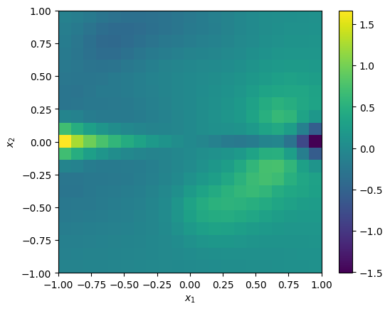
As before, you can also evaluate light weighted quantities e.g. to evaluate a skewness map of the light-weighted LOSVDs,

skew_v_x = galaxy.get_skewness('v_x', light_weighted=True)
_ = cube.imshow(skew_v_x)

L-Moments

In addition to standard moments, popkinmocks offers the option to calculate L-moments. These are robust alternatives to conventional moments based on order statistics. They can be evaluated similarly to standard moments, via the methods:

• get_l_mean,

• get_l_variance,

• get_l_skewness,

• get_l_kurtosis, or get_excess_l_kurtosis,

while the method get_excess_l_moment can be used for arbitrary higher orders.

To see why we need more robust alternatives to conventional moments, consider the following. Let’s create copy of our example galaxy (using the a base component class), where we slightly perturb the underlying density. Specifically, we add a density spike for large negative velocities in spaxel \((5,5)\):

log_p_tvxz = galaxy.get_log_p('tvxz')
log_p_tvxz[:,0,5,5,:] += 21. # add density to leftmost velocity bin, spaxel (5,5)
gal_perturbed = pkm.components.Component(cube=cube, log_p_tvxz=log_p_tvxz)

The resulting change to the velocity distributions is the (barely visible) spike on the leftmost side of this plot:

p_v_x = galaxy.get_p('v_x')
p_v_x_perturbed = gal_perturbed.get_p('v_x')
cube.plot('v', p_v_x[:,5,5])
cube.plot('v', p_v_x_perturbed[:,5,5], '--', label='perturbed')
_ = plt.legend()

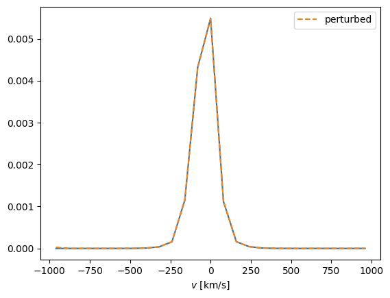
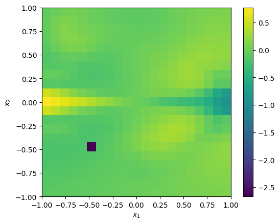
Though this spike is barely visible, the resulting change in the velocity skewness at that position is substantial compared to before:

skew_v_x_perturbed = gal_perturbed.get_skewness('v_x', light_weighted=True)
_ = cube.imshow(skew_v_x_perturbed)

The L-skewness, on the other hand, is far more robust to this small perturbation:

l_skew_v_x = galaxy.get_l_skewness('v_x', light_weighted=True)
l_skew_v_x_perturbed = gal_perturbed.get_l_skewness('v_x', light_weighted=True)

fig, ax = plt.subplots(1,2)
cube.imshow(l_skew_v_x, ax=ax[0], colorbar=False, label_ax=False)
cube.imshow(l_skew_v_x_perturbed, ax=ax[1], colorbar=False, label_ax=False)
ax[0].set_title('L-skewness, original')
_ = ax[1].set_title('L-skewness, perturbed')

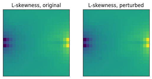
This robustness derives from the fact that L-moments are linear statistics, as opposed to higher-order statistics such as skewness which is cubic in the abscissa values. Perturbations such as the one we have manually inserted here can more realistically arise when the density is reconstructed from observed, noisy data. In these cases, L-moments may be preferred to the conventional moments.

Covariances and Correlations

Covariances and correlation are quantities which encode the degree of relation between two variables. The methods get_covariance and get_correlation can evaluate these quantities for any bivariate (marginal or conditional) distribution.

A map of the covariance between stellar age and metallicity for example is given by

\[ \mathbb{Cov}(t,z|x) = \int (t-\mathbb{E}(t|x)) (z-\mathbb{E}(z|x)) p(t,z|x) \;\mathrm{d}t \;\mathrm{d}z. \]

To calculate this, do this

covar_tz_x = galaxy.get_covariance('tz_x')

To instead get the correlation instead of the covariance, i.e.

\[ \mathbb{Cor}(t,z|x) = \frac{\mathbb{Cov}(t,z|x)}{\sqrt{\mathbb{Var}(t|x)\mathbb{Var}(z|x)}} \]

do this,

correlation_tz_x = galaxy.get_correlation('tz_x')

The correlation should be normalised to be between -1 and 1,

np.max(np.abs(correlation_tz_x)) <= 1.

np.True_

Rules for constructing valid input strings are similar to those given above, except the target distribution must be bivariate, i.e. have exactly two dependent parameters.

As with 1D moments, if one of the dependent variables is x then the first dimension of the output stacks the covariances over \(x_1\) and \(x_2\), i.e.

covar_vx = galaxy.get_covariance('vx')
# covar_vx[0] = Cov(v,x_1)
# covar_vx[1] = Cov(v,x_2)

Light or Mass Weighting

By default, popkinmocks deals with mass-weighted quantities. When we say the density \(p(t, v, \textbf{x}, z)\) is mass-weighted, this means that if you integrate it over some volume in \((t, v, \textbf{x}, z)\) space, the result is equal to the fraction of stellar mass in that volume. The light-weighted distribution, on the other hand, would return the fraction of stellar light.

Mass-weighted and light-weighted quantities are different because different stellar populations have different integrated luminosities,

\[ \mathcal{L}(t,z) = \int S(\lambda ; t, z) \;\mathrm{d}t \;\mathrm{d}z \]

ssps = pkm.model_grids.milesSSPs()
ssps.get_light_weights()

from matplotlib.colors import LogNorm

ax = cube.imshow(
  ssps.light_weights,
  view=['t','z'],
  norm=LogNorm(),
  colorbar_label='$\mathcal{L}(t,z)$'
  )
_ = ax.set_title('Integrated Flux of SSPs')

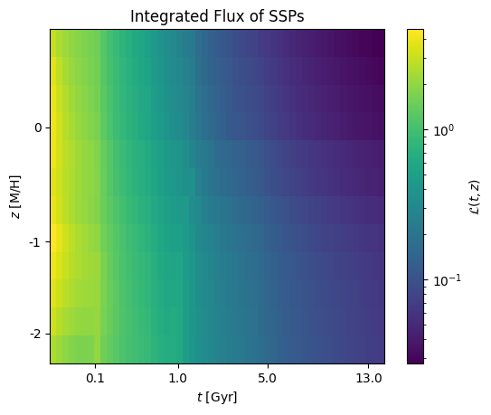
This varies strongly with age - young stars are much brighter than old stars - and weakly with metallicity.

We get the light-weighted density \(p_\mathcal{L}(t, v, \textbf{x}, z)\) from the mass-weighted version by scaling by light weights and appropriately normalising, i.e.

\[ p_\mathcal{L}(t, v, \textbf{x}, z) \propto \mathcal{L}(t,z) p(t, v, \textbf{x}, z). \]

This \(p_\mathcal{L}(t, v, \textbf{x}, z)\) forms the basis for all light-weighted calculations. All methods to evaluate probability functions and moments can accept the argument light_weighted=True.