Constructing Models

popkinmocks offers several options to construct models:

• from simulation particles (FromParticle),

• using a library of parameterised components (ParametricComponent),

• as a mixture of other components (Mixture),

• from a pixel representation of \(p(t, v, \textbf{x}, z)\) (using the base Component class),

• save and load existing models from file (using dill).

The first four options are related via the following inheritance diagram:

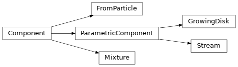
Parameterised components are based on simple analytic equations while simulations can provide more physically self-consistent models. Different types of components have customised methods to improve various calculations e.g.:

• we use exact expressions for Fourier transforms to evaluate datacubes for parameterised components,

• we use exact expressions to evaluate moments for mixture components.

This notebook will demonstrate each option. To ensure that these examples run quickly when building the documentation, we will restrict the size of the problem to something manageable: we thin the parameters of our SSP grid, and use fairly coarse spatial and velocity discretisations for the cube:

import numpy as np
np.random.seed(881230)
np.seterr(divide='ignore', invalid='ignore') # hide some warnings
import matplotlib.pyplot as plt

import popkinmocks as pkm

ssps = pkm.milesSSPs(thin_age=6, thin_z=2)
cube = pkm.ifu_cube.IFUCube(
  ssps=ssps, nx1=21, nx2=21, nv=25, vrng=(-1000,1000)
  )

Simulation data

Let’s create some random toy data representing (equal-mass) stellar particle data from a simulation:

N = 10000
t = np.random.uniform(0, 13, N) # age [Gyr]
v = np.random.normal(0, 200., N) # LOS velocity [km/s]
x1 = np.random.normal(0, 0.4, N) # x1 position [arbitary]
x2 = np.random.normal(0, 0.2, N) # x2 position [arbitary]
z = np.random.uniform(-2.5, 0.6, N) # metallicty [M/H]

You can create a popkinmocks component from this data as follows,

Note

If particles aren’t equal-mass, use the mass_weights argument of FromParticle.

simulation = pkm.components.FromParticle(cube, t, v, x1, x2, z)

Note: 903/10000 particles out of bounds.
N lost	: low/high
   t	: 0/0
   v	: 0/0
   x1	: 61/49
   x2	: 0/0
   z	: 0/800

The output tells you how many particles have been ignored as they fall outside our variable limits e.g. here 800 particles had a metallicity above the upper bound of our SSP grid and will not enter into any subsequent calculations.

We can evaluate the datacube \(\bar{y}\) for this component,

simulation.evaluate_ybar()
simulation.ybar.shape

(1215, 21, 21)

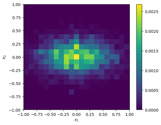
This shape corresponds to our sampling in (log) wavelength and spatial dimensions. We could produce an image by summing over wavelength,

image = np.sum(simulation.ybar, 0)
_ = cube.imshow(image)

or look at the spatially-integrated spectrum by summing over both spatial dimensions,

integrated_spectrum = np.sum(simulation.ybar, (1,2))
_ = cube.plot_spectrum(integrated_spectrum)

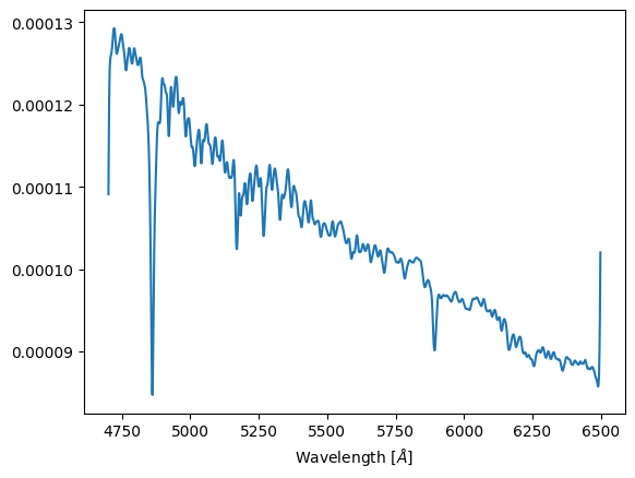
The large spikes at the start and end of this spectrum are unphysical artifacts - see FAQs for more info.

Parameterised components

The base ParametricComponent class arises from assuming (i) a specific factorisation of \(p(t, v, \textbf{x}, z)\), and (ii) specific functional forms for factors of \(p(t, v, \textbf{x}, z)\).

The assumed factorisation is,

\[ p(t, v, \textbf{x}, z) = p(t) p(\textbf{x}|t) p(v|t,\textbf{x}) p(z|t,\textbf{x}) \tag{1} \label{eq:factor_p} \]

The velocity factor \(p(v|t,\textbf{x})\) depends on stellar age and position but not on metallicity. This is a simplifying assumption we have used to speed up evaluation of datacubes for ParametricComponents.

The remaining assumptions are specific choices of the factors in \(\eqref{eq:factor_p}\). Some of these are shared across all instances of ParametricComponent, while some are implemented for individual subclasses (i.e. GrowingDisk or Stream):

• \(p(t)\) is a beta distribution,

• \(p(\textbf{x}|t)\) implemented in subclasses,

• \(p(v|t,\textbf{x}) = \mathcal{N}(v ; \mu_v(\textbf{x},t),\sigma_v(\textbf{x},t))\),

  • the functions \(\mu_v(\textbf{x},t)\) and \(\sigma_v(\textbf{x},t)\) implemented in subclasses,

• \(p(z|t,\textbf{x})\) from chemical enrichment model in Zhu et al. 20 (Section 3),

  • depends on a spatially varying depletion timescale \(t_\mathrm{dep}(\textbf{x})\)

  • i.e. \(p(z|t,\textbf{x}) = p(z|t;t_\mathrm{dep}(\textbf{x}))\)

  • the function \(t_\mathrm{dep}(\textbf{x})\) implemented in subclasses

To give you a feel for this chemical evolution model, here are three age-metallity distributions for different depletion timescales:

fig, ax = plt.subplots(1, 3)
parametric_cmp = pkm.components.parametric.ParametricComponent(cube=cube)

for t_dep, ax0 in zip([0.5, 5., 13.], ax):
  p_z_t = parametric_cmp.evaluate_chemical_enrichment_model(t_dep)
  cube.imshow(p_z_t.T, view=['t', 'z'], colorbar=False, ax=ax0)
  ax0.set_title('$t_\mathrm{dep} = '+str(t_dep)+'$ Gyr')

fig.tight_layout()

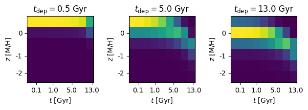
You can see that for a larger \(t_\mathrm{dep}\), enrichment (i) is suppressed to lower overall metallicities, (ii) proceeds more slowly, and (ii) has a larger metal spread at fixed age.

Here I’ll demonstrate the two types of ParametricComponent currently implemented: GrowingDisk and Stream.

GrowingDisk

Initialise the disk component,

disk = pkm.components.GrowingDisk(cube=cube, rotation=0., center=(0,0))

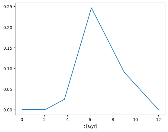
and set its star formation history \(p(t)\). This is a beta distribution parameterised with mean 0<phi<1 and concentration lmd,

disk.set_p_t(lmd=30., phi=0.5)
_ = cube.plot('t', disk.get_p('t'))

We will next set the spatial, velocity, and metallicity factors of \(\eqref{eq:factor_p}\). To resemble galactic disks, we want elliptical isocontours for all three factors. We therefore chose them to be functions of elliptical radius \(r_q\) with flattening \(q\), i.e.

\[ r_q(\textbf{x}) = \sqrt{x_1^2 + \left( \frac{x_2}{q} \right)^2}. \]

and the associated angle

\[ \theta_q(\textbf{x}) = \arctan\left( \frac{x_2}{q} \frac{1}{x_1} \right). \]

In cases where we have age-dependent flattenings \(q=q(t)\), the elliptical radius and angle are also written as functions of age - i.e. as \(r_q(\textbf{x},t)\) and \(\theta_q(\textbf{x},t)\).

Several parameters of the GrowingDisk component will depend on stellar age e.g. age-dependent flattenings \(q=q(t)\). In general, any age-dependent parameter is specified as a pair of values for (young, old) stars and linearly interpolated for intermediate ages e.g.

q_young, q_old = 0.2, 0.8
q_interpolated = disk.linear_interpolate_t(q_young, q_old)
_ = cube.plot('t', q_interpolated)

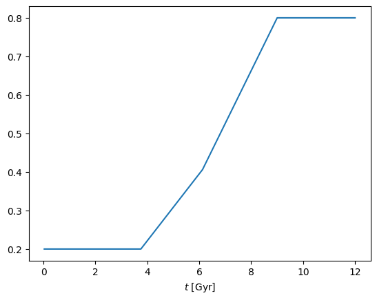
Note that the interpolated quantity is kept constant beyond certain age limits. These limits are automatically set, and are equal to the 5th and 95th percentiles of the star formation history \(p(t)\).

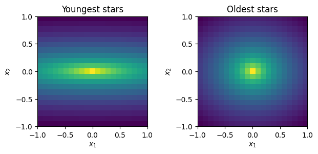
We now set the age dependent spatial density \(p(\textbf{x}|t)\). This is given by a cored power-law,

\[ p(\textbf{x}|t) \propto \left\{r_q(\textbf{x},t) + r_c(t)\right\}^{-\alpha(t)}, \]

which depends on three functions: core length \(r_c(t)\), power-law slope \(\alpha(t)\) and flattening \(q(t)\). We set these,

disk.set_p_x_t(
  q_lims=(0.2, 0.8), # young disk flatter than old
  rc_lims=(0.5, 0.2), # young disk larger core than old
  alpha_lims=(1.2, 0.8) # young disk steeper than old
  )

and we can then evaluate \(p(\textbf{x}|t)\),

p_x_t = disk.get_p('x_t')
print(p_x_t.shape)

(21, 21, 9)

and plot images of the surface density of stars of different ages,

from matplotlib.colors import LogNorm
fig, ax = plt.subplots(1, 2)

cube.imshow(p_x_t[:,:,0], ax=ax[0], norm=LogNorm(), colorbar=False)
ax[0].set_title('Youngest stars')

cube.imshow(p_x_t[:,:,-1], ax=ax[1], norm=LogNorm(), colorbar=False)
_ = ax[1].set_title('Oldest stars')

fig.tight_layout()

Next set the depletion timescale \(t_\mathrm{dep}(\textbf{x})\) for metal enrichment. This is parametrised as

\[ t_\mathrm{dep}(\textbf{x}) = t_\mathrm{dep}^\mathrm{in} + (t_\mathrm{dep}^\mathrm{out} - t_\mathrm{dep}^\mathrm{in}) \left( \frac{r_q(\textbf{x})}{\max(|x_1|)} \right)^{\alpha}, \]

which takes four parameters: flattening \(q\), exponent \(\alpha\), and inner/outer values \(t_\mathrm{dep}^\mathrm{in}\) and \(t_\mathrm{dep}^\mathrm{out}\).

disk.set_t_dep(q=0.5, alpha=1., t_dep_in=1., t_dep_out=7.)
_ = cube.imshow(
  disk.t_dep, 
  cmap=plt.cm.jet, 
  colorbar_label='$t_\mathrm{dep}$ [Gyr]')

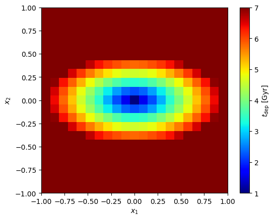
Here we see \(t_\mathrm{dep}^\mathrm{in}\) increase linearly (since \(\alpha=1\)) from \(t_\mathrm{dep}^\mathrm{in}\) at the center to \(t_\mathrm{dep}^\mathrm{out}\) at the edge of the \(x_1\) axis, and then remain constant beyond. We can now evaluate \(p(z|t,\textbf{x})\):

p_z_tx = disk.get_p('z_tx')
print(p_z_tx.shape) # = (nz, nt, nx1, nx2)

(6, 9, 21, 21)

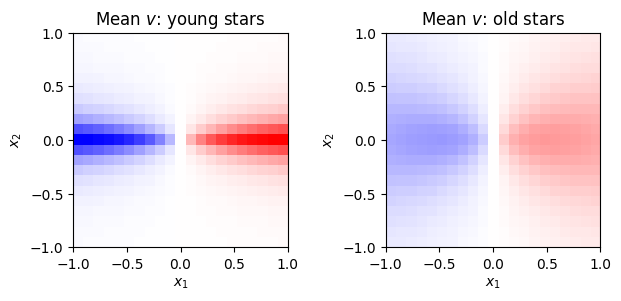
Lastly, set the kinematics via the functions \(\mu_v(\textbf{x},t)\) and \(\sigma_v(\textbf{x},t)\).

The function \(\mu_v(\textbf{x},t)\) resembles the velocity field of a rotating disk. Along the major-axis, the velocity is given by a rotation curve which peaks at some given radius. Off of the major-axis, we turn the 1D rotation curve to a 2D velocity field by multiplying by the cosine of the (flattened) polar co-ordinate \(\theta_q(\textbf{x},t)\). Altogether, this parameterisation requires three (age-dependent) parameters: flattening \(q(t)\), peak velocity \(v_\mathrm{max}(t)\), and the radius at which rotation curve reaches the peak \(r_\mathrm{max}(t)\). The specific function used is,

\[ \mu_v(\textbf{x},t) = v_\mathrm{max}(t) \cos \theta_q(\textbf{x},t) \left( \frac{r_\mathrm{max}(t) + r_c(t)}{r_q(\textbf{x},t) + r_c(t)} \right)^3 \frac{r_q(\textbf{x},t)}{r_\mathrm{max}(t)}. \]

We can set these parameters and plot velocity maps for different ages,

disk.set_mu_v(
  q_lims=(0.1, 0.5),
  rmax_lims=(1., 0.5),
  vmax_lims=(250., 100.)
)

fig, ax = plt.subplots(1, 2)

cube.imshow(disk.mu_v[0], ax=ax[0], vmin=-250, vmax=250, colorbar=False, cmap=plt.cm.bwr)
ax[0].set_title('Mean $v$: young stars')

cube.imshow(disk.mu_v[-1], ax=ax[1], vmin=-250, vmax=250, colorbar=False, cmap=plt.cm.bwr)
ax[1].set_title('Mean $v$: old stars')

fig.tight_layout()

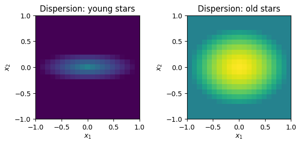
Velocity dispersion \(\sigma_v(\textbf{x},t)\) takes four age-dependent parameters: flattening \(q(t)\), inner and outer values \(\sigma_\mathrm{in}(t)\) and \(\sigma_\mathrm{out}(t)\), and exponent \(\alpha(t)\):

\[ \sigma_v(\textbf{x},t) = \sigma_\mathrm{in}(t) + (\sigma_\mathrm{out}(t) - \sigma_\mathrm{in}(t)) \left( \frac{r_q}{\max(|x_1|)} \right)^{\alpha(t)} \]

We can set these parameters and plot dispersion maps for different ages,

disk.set_sig_v(
  q_lims=(0.3, 0.8),
  alpha_lims=(1.0, 1.8),
  sig_v_in_lims=(100., 200.),
  sig_v_out_lims=(20., 100.))

fig, ax = plt.subplots(1, 2)

cube.imshow(disk.sig_v[0], ax=ax[0], vmin=20., vmax=200, colorbar=False)
ax[0].set_title('Dispersion: young stars')

cube.imshow(disk.sig_v[-1], ax=ax[1], vmin=20, vmax=200, colorbar=False)
ax[1].set_title('Dispersion: old stars')

fig.tight_layout()

Finally we can evaluate the datacube.

disk.evaluate_ybar()

Stream

This is a toy model to resemble stellar streams formed from tidally disrupted satellites. First create the stream and set its star formation history as before:

stream = pkm.components.Stream(cube=cube)
stream.set_p_t(lmd=4., phi=0.9)

Tidal stripping may disrupt spatial structures formed through in-situ star formation. For example age gradients in a satellite galaxy may be mixed away as a stream is formed. This motivates several simplifying assumptions for our stream component:

1. we use a constant depletion timescale, i.e.

\[ t_\mathrm{dep}(\textbf{x}) = t_\mathrm{dep} \]

stream.set_t_dep(0.7)

2. we use a constant velocity dispersion for all positions and ages, i.e.

\[ \sigma_v(\textbf{x},t) = \sigma_v \]

stream.set_sig_v(50.)

3. we remove the age-dependence of spatial density, i.e.

\[ p(\textbf{x}|t) = p(\textbf{x}) \]

4. and we remove the age dependence of mean velocity

\[ \mu_v(\textbf{x},t) = \mu_v(\textbf{x}). \]

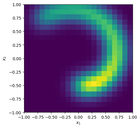
Our choice of \(p(\textbf{x})\) is a curve in polar co-ordinates. This is parameterised with start/end polar angles theta_lims, radii mu_r_lims, and a spatial thickness sig perpendicular to the stream track. Stream radius increases linearly between the given angles. Density along the stream remains constant with polar angle.

stream.set_p_x_t(
  theta_lims=(-np.pi/2., 3*np.pi/4.),
  mu_r_lims=(0.5, 1.),
  sig=0.15
  )

p_x = stream.get_p('x')
_ = cube.imshow(p_x, colorbar=False)

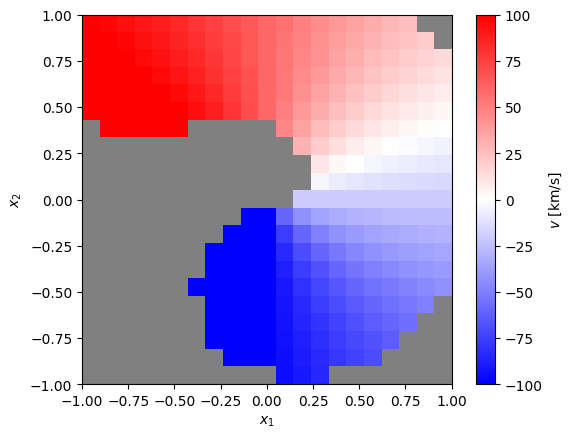
Lastly, the mean velocity \(\mu_v(\textbf{x})\). This varies linearly with polar angle from specified start and end values,

stream.set_mu_v(mu_v_lims=[-100, 100])
mean_v_map = stream.get_mean('v_x')

# plot, masking out regions where stream desnity is low
mask = np.where(p_x < 0.01)
mean_v_map[mask] = np.nan
cmap = plt.cm.bwr.copy()
cmap.set_bad('grey')
_ = cube.imshow(
  mean_v_map, 
  vmin=-100, vmax=100, 
  cmap=cmap, colorbar_label='$v$ [km/s]')

Finally, evaluate the datacube.

stream.evaluate_ybar()

Mixture

These are weighted mixtures of other components. The weights must be non-negative and add to one. For example, to combine the disk and stream component we created above,

mixture = pkm.components.Mixture(
  cube=cube,
  component_list=[disk, stream],
  weights=[0.9, 0.1]
  )
mixture.evaluate_ybar()  

Mixture models are a good way to build complexity as they can have complex moments maps. For example, the skewness of the velocity distribution \(p(v|\textbf{x})\),

skew_v_map = mixture.get_skewness('v_x')
cube.imshow(
  skew_v_map, 
  cmap=plt.cm.bwr, colorbar_label='Skewness')
_ = plt.gca().set_title('Mixture model: skewness of $p(v|x)$')

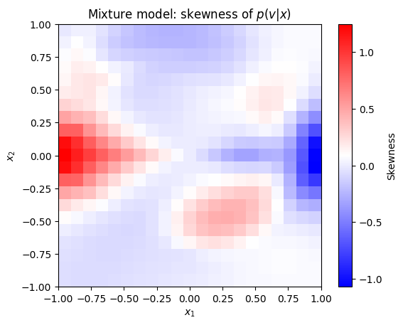
shows the stream clearly superimposed across the disk.

Pixel representation of \(p(t, v, \textbf{x}, z)\)

Another option to create a model is to directly from a pixelated representation of \(p(t, v, \textbf{x}, z)\). This can be done with the base Component class. For better numerical precision, we actually use the log density \(\log p(t, v, \textbf{x}, z)\) instead of the density itself.

But how might you come across a pixelated representation of \(\log p(t, v, \textbf{x}, z)\)? One option is to create a histogram of simulation particles, then take its logarithm. This is exactly what is implemented in the FromParticle class.

Another way you could access a \(\log p(t, v, \textbf{x}, z)\) is by using another popkinmocks component. For example we can create a pixelated version of the mixture model,

log_p_tvxz = mixture.get_log_p('tvxz')
pixel_copy = pkm.components.Component(cube=cube, log_p_tvxz=log_p_tvxz)

You can then compare quantities calculated using the original mixture model and this pixelated version. Differences may arise due to numerical errors. If we compare the two datacubes for example,

pixel_copy.evaluate_ybar()
error = pixel_copy.ybar - mixture.ybar
error_pc = 100.*error/mixture.ybar
median_abs_err = np.median(np.abs(error_pc))
print(f'Median abolsute error = {median_abs_err:.2f} %')

Median abolsute error = 0.04 %

we see the error is small. If we compare the skewness map we calculated earlier however,

error = pixel_copy.get_skewness('v_x') - skew_v_map
error_pc = 100.*error/skew_v_map
median_abs_err = np.median(np.abs(error_pc))
print(f'Median abolsute error = {median_abs_err:.2f} %')

Median abolsute error = 7.77 %

we see are significant differences. Increasing the velocity resolution of the cube (nv) should reduce these errors. Checks such as these form the basis of the automated testing routines in popkinmocks.

From file using dill

We use the dill package to save and load files. Components have a convenicence method dill_dump to save into a .dill file. For example, to save the mixture component we made previously,

mixture.dill_dump(fname='my_mixture_component.dill', direc='data/')

This can then be reloaded in a later session,

import dill
with open('data/my_mixture_component.dill', 'rb') as file:
    mixture_reloaded = dill.load(file)
print(mixture_reloaded)

<popkinmocks.components.mixture.Mixture object at 0x7f51c4cd2b10>