FAQs

import numpy as np
import matplotlib.pyplot as plt
import popkinmocks as pkm

ssps = pkm.milesSSPs()
cube = pkm.ifu_cube.IFUCube(ssps=ssps, nx1=10, nx2=10, nv=21)

Why does my spectrum start and end with spikes?

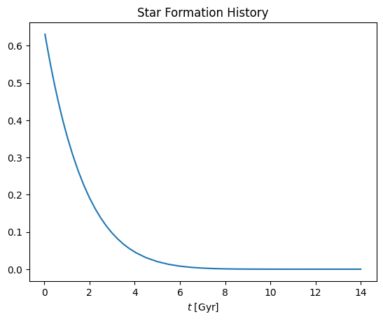
Let’s create a component with lots of young stars and a broad LOSVD (leaving other settings at their defaults):

s = pkm.components.Stream(cube=cube)
s.set_p_t(lmd=10., phi=0.1)
s.set_sig_v(300.)
s.set_t_dep()
s.set_p_x_t()
s.set_mu_v()

cube.plot('t', s.get_p('t'))
_ = plt.gca().set_title('Star Formation History')

If we evaluate the datacube of this component and plot the integrated spectrum,

s.evaluate_ybar()
integrated_spectrum = np.sum(s.ybar, (1,2))
_ = cube.plot_spectrum(integrated_spectrum)

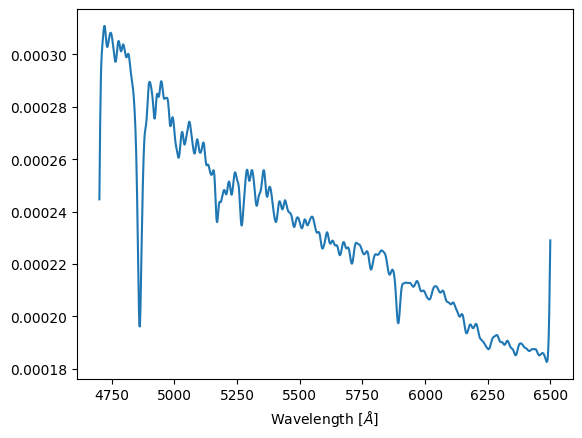
we see large spikes the start and end. These are not spectral lines. They are unphysical artifacts which arise because we use Fourier transforms to perform convolutions. This implicitly assumes that the LOSVD is periodic, and results in the endpoints of the spectrum wrapping around. This effect is most visible when the model contains a significant amount of young stars (which have a steep continuum) with a broad LOSVD. Even when not so clearly visible, however, this effect is always present and should be masked out for subsequent analyses.

How should I contruct a mask to deal with wrapping around?

To construct a mask we must have an estimate of the width of the LOSVD. Broader LOSVDs will result in more wrapping around. So pick some maximum absolute velocity that you are confident contains all the LOSVD, i.e. pick some \(v_\mathrm{max}\) where you are confident that

\[ \int_{-v_\mathrm{max}}^{v_\mathrm{max}} p(v) \; d\mathrm{v} \approx 1 \]

Then convert this to a mask for spectral fitting as follows:

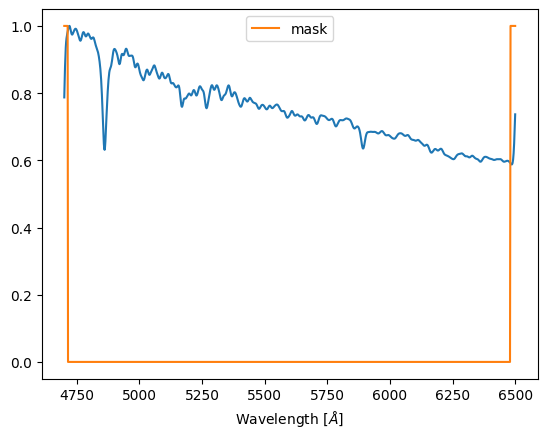
v_max = 1000.
n_spaxels_to_mask = int(v_max/cube.ssps.dv)
mask = np.zeros_like(integrated_spectrum, dtype=int)
mask[:n_spaxels_to_mask] = 1
mask[-n_spaxels_to_mask:] = 1

# normalise spectrum for plotting
integrated_spectrum /= np.max(integrated_spectrum)
cube.plot_spectrum(integrated_spectrum)
cube.plot_spectrum(mask, label='mask')
_ = plt.gca().legend()