Background#

This introduction provides some background about stellar populations, kinematics and the forward model to evaluate the integrated-light stellar contribution to IFU datacubes.

Stellar populations and kinematics#

popkinmocks describes the stellar content of galaxies as a joint probability distribution \(p(t, v, \textbf{x}, z)\) over four variables:

age \(t\),
line-of-sight (LOS) velocity \(v\),
2D on-sky position \(\mathbf{x}\), and
metallicity \(z\).

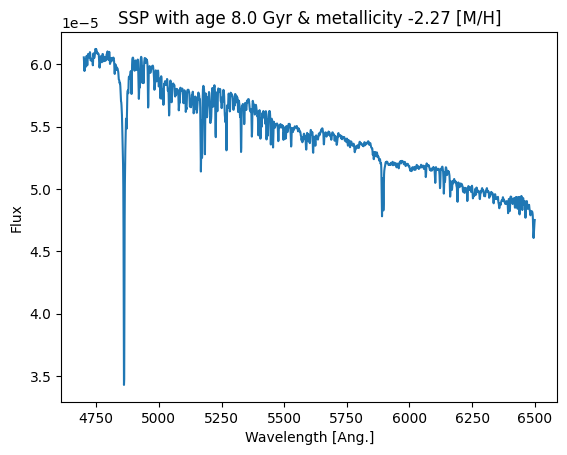
A simple (AKA single) stellar population (SSP) is a population of stars born at the same time and having the same initial chemical composition. In popkinmocks we use the (MILES models) to represent the spectra of SSPs. Let’s look at the spectrum of one SSP:

import popkinmocks as pkm
import matplotlib.pyplot as plt

ssps = pkm.model_grids.milesSSPs()

# plot ssp for a given model index
index = 40
t, z, spectrum = ssps.get_ssp(index)
_ = plt.plot(ssps.lmd, spectrum)
_ = plt.gca().set_title(f'SSP with age {t} Gyr & metallicity {z} [M/H]')
_ = plt.gca().set_xlabel('Wavelength [Ang.]')
_ = plt.gca().set_ylabel('Flux')

../_images/178d91f1d760cc2a8d772524fae371eba96e332777b85931736dcbf36b5142de.png

Stellar kinematics refer to the velocities and positions of stars within a galaxy. The joint distribution \(p(t, v, \textbf{x}, z)\) encodes a complete description of the relations between stellar population and kinematic variables.

IFU datacubes#

Integral Field Units (IFUs) are a type of instrument which can observe spatial and spectral information simultaneously. IFU observations result in datacubes \(y(\textbf{x}, \lambda)\) which describe the flux observed at a position \(\textbf{x}\) and wavelength \(\lambda\). The datacube is connected to the stellar population-kinematic distribution via the equation:

\[ \begin{equation} y(\textbf{x}, \lambda) = \int \int \int \frac{1}{1+v/c} p(t, v, \textbf{x}, z) S\left(\frac{\lambda}{1+v/c} ; t, z\right) \; \mathrm{d}t \; \mathrm{d}v \; \mathrm{d}z \tag{1} \label{eq:fwdmod} \end{equation} \]

where we have introduced notation for the:

spectrum of SSP with age \(t\) and metallicity \(z\), \(S(\lambda ; t, z)\), and
speed of light, \(c\).

The two factors of \((1+v/c)\) in this equation arise from Doppler-shifting of light: the factor inside \(S\) translates from the rest-frame to observed wavelengths given a LOS velocity \(v\), while the pre-factor scales the flux, ensuring total luminosity is conserved.

How is this connected to spectral modelling?#

By describing stellar populations and kinematics simultaneously via the joint distribution \(p(t, v, \textbf{x}, z)\) we can encode complex relations between these four variables without imposing simplifying assumptions. One such assumption which is commonly used when modelling observed spectra is that at a fixed position, velocities and stellar populations are independent. This statement is equivalent to the factorisation:

\[ p(t, v, \textbf{x}, z) = p(\textbf{x}) p(v|\textbf{x}) p(t,z|\textbf{x}) \tag{2} \label{eq:factor_p} \]

which says that velocities and stellar populations only interact via their dependence on position.

What happens if we insert the simplifying assumption shown in \(\eqref{eq:factor_p}\) into the integral equation for the datacube i.e. equation \(\eqref{eq:fwdmod}\)? In this case, the integral can be factored as follows

\[ \begin{equation} y(\textbf{x}, \lambda) = p(\textbf{x}) \int \frac{p(v|\textbf{x})}{1+v/c} \left[\int \int p(t,z|\textbf{x}) S\left(\frac{\lambda}{1+v/c} ; t, z\right) \; \mathrm{d}t \; \mathrm{d}z \right] \;\mathrm{d}v . \end{equation} \]

This is the forward-model is used in most typical analyses of binned spectra from IFU datacubes i.e. a binned spectrum extracted at a position \(\textbf{x}\) is modelled as a superposition of SSPs weighted by \(p(t,z|\textbf{x})\) and convolved with a single line-of-sight velocity distribution (LOSVD) \(p(v|\textbf{x})\) which is independent of stellar populations.

Evaluating datacubes using FFTs#

popkinmocks evaluates equation \(\eqref{eq:fwdmod}\) to produce datacubes for a given choice of \(p(t, v, \textbf{x}, z)\). To help perform the integral over \(v\), popkinmocks uses the fact that \(\eqref{eq:fwdmod}\) can be re-written as a standard convolution by changing variables:

log wavelength, \(\omega = \ln \lambda\)
transformed velocity, \(u = \ln(1 + v/c)\).

This transforms \(\eqref{eq:fwdmod}\) into a standard convolution over \(u\):

\[ \begin{equation} \tilde{y}(\textbf{x}, \omega) = \int \int \int \tilde{p}(t, u, \textbf{x}, z) \tilde{S}\left(\omega - u; t, z\right) \; \mathrm{d}t \; \mathrm{d}u \; \mathrm{d}z \label{eq:fwdmod_transformed} \end{equation} \]

where \(\tilde{y}\), \(\tilde{p}\) and \(\tilde{S}\) are minor labellings of \(y, p\) and \(S\) (see Section 2.2.1 of Ocvirk et. al for details). popkinmocks evaluates this convolution using a Fast Fourier Transform (FFT), producing a datacube sampled in log wavelength \(\omega\) rather than wavelength \(\lambda\).

Discretisation#

popkinmocks perfroms calculations using discrete approximations to the continuous variables \((t, v, \textbf{x}, z)\). The discretisation in \(t\) and \(z\) is set by the SSP grid; there are options available when instantiating SSP models which control this grid e.g.

ssps = pkm.milesSSPs(thin_age=3, z_lim=(-1, 0), lmd_min=5000, lmd_max=6000)

Discretisation in the spatial dimensions \(\textbf{x}=(x_1, x_2)\) and velocity \(v\) are chosen when instantiating the IFUCube object,

cube = pkm.ifu_cube.IFUCube(
  ssps=ssps, 
  nx1=20, x1rng=(-1,1),      # arbitrary units
  nx2=21, x2rng=(-1,1),      # arbitrary units
  nv=30, vrng=(-1000,1000)   # km/s
)

The shape of the discretisation in all variables is given by

cube.get_distribution_shape('tvxz')

which corresponds to the size of each variable in the string tvxz i.e. \((t, v, x_1, x_2, z)\). To get the values of metallicity,

cube.get_variable_values('z')

array([-0.96  , -0.6575, -0.4025, -0.25  ])

and likewise for the other variables.

Background

Contents