Observation Noise#
Here we present noise models available in popkinmocks. Noise \(\epsilon\) is added to the signal \(\bar{y}\) to give the observed cube \(y_\mathrm{obs}\),
Currently we assume that noise is un-correlated between spaxels and Gaussian i.e. \(\epsilon(\mathbf{x},\omega)\) is sampled from a normal distribution with variance \(\sigma(\mathbf{x},\omega)^2\),
We provide two models for \(\sigma(\mathbf{x},\omega)\). To demonstrate these, I’ll use the mixture model we saved on the Constructing Models page:
import numpy as np
np.random.seed(301288)
import matplotlib.pyplot as plt
import dill

import popkinmocks as pkm

with open('data/my_mixture_component.dill', 'rb') as file:
    galaxy = dill.load(file)
cube = galaxy.cube
Constant SNR#
This implements a constant signal-to-noise ratio (SNR), i.e.
constant_snr = pkm.noise.ConstantSNR(galaxy)
yobs_const_snr = constant_snr.get_noisy_data(snr=100)
Shot noise#
This model is more realistic. Motivated by Poisson/shot noise, here the noise standard deviation scales as the square root of the signal, i.e.
The constant of proportionality is chosen so that a desired maximum signal-to-noise ratio is achieved in the brightest voxel, i.e.
shot_noise = pkm.noise.ShotNoise(galaxy)
yobs_shot_noise = shot_noise.get_noisy_data(snr=100)
Comparison#
def plot_spectrum_from_pixel(i, j, ax):
  cube.plot_spectrum(galaxy.ybar[:,i,j], '-', ax=ax, label='$\\bar{y}$')
  cube.plot_spectrum(yobs_const_snr[:,i,j], '.', ax=ax, label='ConstantSNR')
  cube.plot_spectrum(yobs_shot_noise[:,i,j], '.', ax=ax, label='ShotNoise')
  ax.legend()
  ax.set_xlim(5800, 6000)
  ax.set_yticks([])

fig, ax = plt.subplots(1,2)
plot_spectrum_from_pixel(10, 10, ax=ax[0])
ax[0].set_title('Inner, bright pixel')
plot_spectrum_from_pixel(0, 0, ax=ax[1])
ax[1].set_title('Outer, faint pixel')
fig.tight_layout()
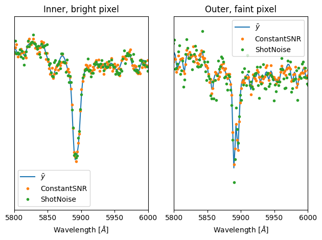
In the bright central pixel (left) the SNRs of the two noise models are equal, both with SNR=100. At the outer pixel (right) the SNR of the ShotNoise model has decreased in line with the decreased flux, while for ConstantSNR the SNR remains high.